ANN - Back Propagation of Errors

The first training algorithm which - historically speaking - was able to deal with hidden layers in neural networks is called the "back propagation of errors". It is used for modifying the weights of multi-layer perceptrons, which have an input layer, a hidden layer, and an output layer. Note that multi-layer perceptrons are often dubbed "back propagation networks", which points to the enormous influence this algorithm had on the development of neural networks.

The basic principles of the back propagation algorithm are:

1. the error of the output signal of a neuron is used to adjust its weights such that the error decreases, and
2. the error in hidden layers is estimated proportional to the weighted sum of the (estimated) errors in the layer above.

During the training, the data is presented to the network several thousand times. For each data sample, the current output of the network is calculated and compared to the "true" target value. The error signal δ_j of neuron j is computed from the difference between the target and the calculated output. For hidden neurons, this difference is estimated by the weighted error signals of the layer above. The error terms are then used to adjust the weights w_ij of the neural network.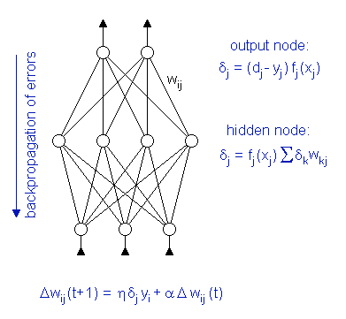

Thus, the network adjusts its weights after each data sample. This learning process is in fact a gradient descent in the error surface of the weight space - with all its drawbacks. The learning algorithm is slow and prone to getting stuck in a local minimum.

For the standard back propagation algorithm, the initial weights of the multi-layer perceptron have to be relatively small. They can, for instance, be selected randomly from a small interval around zero. During training they are slowly adapted. Starting with small weights is crucial, because large weights are rigid and cannot be changed quickly.

The following  interactive example  shows how a multi-layer perceptron learns to model data.