| Fundamentals of Statistics contains material of various lectures and courses of H. Lohninger on statistics, data analysis and chemometrics......click here for more. |

|
Home  Multivariate Data Modeling Neural Networks Recurrent Networks Multivariate Data Modeling Neural Networks Recurrent Networks |
|
| See also: ANN - Introduction, Time Series Processing |   |
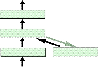
ANN - Recurrent NetworksNetworks with feedback loops belong to the group of recurrent networks. There, unit activations are not only delayed while being fed forward through the network, but are also delayed and fed back to preceding layers. This way, information can cycle in the network. At least theoretically, this allows an unlimited number of past activations to be taken into account. Practically, the influence of past inputs decays rapidly, because it is merged with new ones. The speed of decay can be tuned, but after a few time steps, past information cannot be recognized anymore. Recurrent networks should be trained by some training algorithm propagating the error back through time. This is the consequence of a sequence of past inputs having an influence on later outputs. This technique can be visualized by unfolding the network in time [Hertz et al., 1991]. It is used by the BPTT (Back Propagation Through Time) algorithm. Since the effort of propagating the error back through time is quite high, the temporal aspect is often ignored during training. Simple Recurrent Networks:A typical example of a simple recurrent network is the Elman network. It keeps a copy of the hidden layer for the next updating step. This copy is then used together with the new input. Since
the hidden layer pre-structures the input for the output, it is a valuable
source of information. This explains its success with many forecasting
tasks. Its architecture is shown in the following figure: network. It keeps a copy of the hidden layer for the next updating step. This copy is then used together with the new input. Since
the hidden layer pre-structures the input for the output, it is a valuable
source of information. This explains its success with many forecasting
tasks. Its architecture is shown in the following figure:
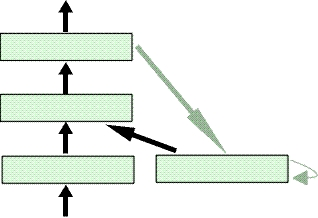
Another example of a simple recurrent network
is the Jordan
Merging can be done by weighting and adding the unit activations. For instance, the activation of a unit in a memory layer at can integrate the output ot-1 as follows: Of course, these weights can be altered. The memory layer can also be regarded as the state of the network. Moreover, multiple techniques for handling sequential information, such as various types of time delays, feedback loops, and memory layers, can be combined to form more powerful temporal neural networks. The strength of such networks is that they combine memories of different length. However, large networks have a large number of degrees of freedom, which makes their training difficult. Fully Recurrent Network:The Fully Recurrent Network (FRN), which is presented by Williams et al., belongs to the group of recurrent networks because it contains several feedback loops. However, it differs from most other approaches.
The layers are arranged differently, and a special training algorithm is
available: the RTRL algorithm (Real Time Recurrent Learning Algorithm).
It traces all activations back through time, which results in very good
solutions. This algorithm is non-local in that single units have access
to the whole network. This conflicts with the idea that the units receive
input solely via the incoming connections. As a result, the tasks of the
units cannot be parallelized. Due to the enormous effort and processing
time required by the RTRL algorithm, the tested Fully Recurrent Networks
are usually rather small and hardly applicable to real-world tasks.
|
|
| Home Multivariate Data Modeling Neural Networks Recurrent Networks |
|