| Fundamentals of Statistics contains material of various lectures and courses of H. Lohninger on statistics, data analysis and chemometrics......click here for more. |

|
Home  Multivariate Data Modeling Classification and Discrimination Classifier Performance Multivariate Data Modeling Classification and Discrimination Classifier Performance |
|||||||||||||||||||||
| See also: Discrimination and Classification, ROC Curve, Predictive Ability |   |
||||||||||||||||||||
Classifier PerformanceEvaluating the performance of a classifier largely depends on the type of classifier. In the most common (and simplest) case we deal with binary classifiers creating only two outcomes. While the methods for the evaluation of binary classifiers are well established and straightforward, the situation with multiclass methods creating more than two possible answers is much more complicated. Furthermore, the situation may become even more difficult if several classifiers are combined to give the final decision. In order to make things simple, the following introduction is restricted to binary classifiers only. When looking at binary classifiers we see that each observation A is mapped to one of two binary labels (e.g. to YES and NO, or 0 and 1, or healthy and sick) upon classification. The classifier response may be either correct or wrong with respect to the (unknown) reality and may be summarized in a confusion matrix, which contains the counts of occurrences of all four possible combinations of classification results. If the response of the classifier is correct then we speak of "true positive" or "true negative" results, depending on the actual class the observation belongs to. If the classifier is wrong upon the true class we speak of "false positive" or "false negative" decisions:
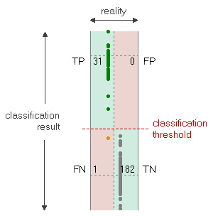
Correct classifications appear in the diagonal elements (green regions), and errors appear in the off-diagonal elements (red regions). Some classifier models (such as discriminant analysis, for example) provide above all a continuous output which has to be compared to a classification threshold in order to deliver a binary result. In the case of a continuous response the confusion matrix may be visualized by plotting the continuous output of the classification model on one axis and the actual class (the "reality") on the other axis. The classification threshold is indicated by a broken line:
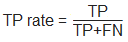
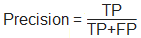
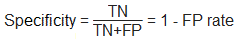
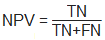
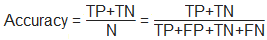
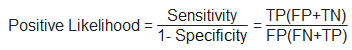
This diagram allows to visually judge the reliability of a classifier simply by looking at the distance and the density of those observations which fall close to the decision threshold. In order to specify the classifier performance in a more formal and quantitative way, several measures have been defined. The table below uses the following notation: N .... total number of observations
|
|||||||||||||||||||||
| Home Multivariate Data Modeling Classification and Discrimination Classifier Performance |
|
||||||||||||||||||||