Filters - Mathematical Background
The process of filtering, which comprises smoothing as a special case,
can be described mathematically in several equivalent ways:
Linear Algebra
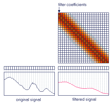
Smoothing can be performed by moving a window over the signal and averaging
data points within the window. In a more general setting it is a weighted
average, where the weighing factors are called filter coefficients. We
can split the weighted average approach into two calculation steps:
-
an element-wise multiplication of the data points with the filter coefficients
-
summing all the weighted points in the window
This is identical to a dot product of two vectors, where one vector consists
of the data points in the window and the other vector of the filter coefficients.
We can include the selection of the window in the dot product by setting
the values for the filter coefficients outside of the window to zero, so
our data vector will be the whole signal. The moving of the window requires
us to use a different vector for the filter coefficients for each move
or shift. This results in a series of vector dot products, which
can be assembled into one matrix multiplication.
Convolution
The mathematical operation of convolution
(often represented by a star) is decribed by the following equation:
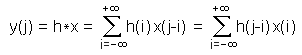 .
Here x is the noisy signal, h stands for the filter coefficients,
y
is the smoothed signal, and
j is the index to the data points, while
i
is the index for the filter coefficients. In the case that we have 2n+1
filter coefficients, the index i runs from -n to +n. So our data
window stretches only n points to the right and left of the data point
under consideration. This approach is computationally more efficient than
the matrix multiplication approach, where the windowing has to be done
by a large number of multiplications by zero. .
Here x is the noisy signal, h stands for the filter coefficients,
y
is the smoothed signal, and
j is the index to the data points, while
i
is the index for the filter coefficients. In the case that we have 2n+1
filter coefficients, the index i runs from -n to +n. So our data
window stretches only n points to the right and left of the data point
under consideration. This approach is computationally more efficient than
the matrix multiplication approach, where the windowing has to be done
by a large number of multiplications by zero.
When we pay close attention, we see that the convolution equation is
for time-reversed filter coefficients, since we multiply h(-n) by x(j-(-n))=x(j+n).
For most of the smoothing filters this has no meaning, since the coefficents
are symmetric around the middle value.
Convolution in the Fourier Domain
It can be shown that the convolution in the Fourier domain can be represented
by the following equation:
 The capitalized variables stand for the Fourier-transformed variables y,
x and h. The frequency is depicted by
ω. In
the Fourier domain convolution reduces to an element-wise multiplication
of the signal and the filter coefficients. H is also called impulse reponse,
since it is obtained by setting the signal x equal to an impulse, i.e.
it is zero everywhere except for one data point that is '1', and convolving
it with h. The Fourier transform of the result of the convolution between
this signal x and h is equal to H and is called impulse reponse.
The capitalized variables stand for the Fourier-transformed variables y,
x and h. The frequency is depicted by
ω. In
the Fourier domain convolution reduces to an element-wise multiplication
of the signal and the filter coefficients. H is also called impulse reponse,
since it is obtained by setting the signal x equal to an impulse, i.e.
it is zero everywhere except for one data point that is '1', and convolving
it with h. The Fourier transform of the result of the convolution between
this signal x and h is equal to H and is called impulse reponse.
State Space Notation
The most general form of describing filters is the so-called state-space
notation:
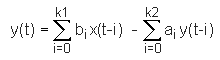 .
It is a generalized version of the convolution equation we gave above.
Here the filter coefficients are given by ai and bi
and the index i runs from 0 to ki instead of -n to +n. The second
sum on the right includes contributions of already filtered data points.
Depending on whether the filter coefficients ai and bi
are zero, the filters have different properties and names. .
It is a generalized version of the convolution equation we gave above.
Here the filter coefficients are given by ai and bi
and the index i runs from 0 to ki instead of -n to +n. The second
sum on the right includes contributions of already filtered data points.
Depending on whether the filter coefficients ai and bi
are zero, the filters have different properties and names.
-
When all the bi coefficients are zero, the filter is called
an
Infinite Impulse Response (IIR) or recursive filter. Auto-regressive
(AR) random processes can be produced by applying this filter to random
inputs.
-
When all the ai coefficients are zero, the filter is called
Finite
Impulse Response (FIR) or non-recursive filter. Moving average (MA)
random processes can be produced by applying this filter to random inputs.
|

 Bivariate Data
