Cauchy Distribution
| Definition |
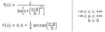
|
| Properties |
- The distribution is symmetric about the parameter a.
- The parameter b determines the width of the distribution
- The central moments are undefined for Cauchy distributed data, which is a consequence of the long tails of the density function (see example below).
- The median and the mode are equal to the location parameter a.
- The standard Cauchy distribution is given by the parameters a=0 and b=1, and is equal to a t distribution having one degrees of freedom.
|
| Graphic Representation |
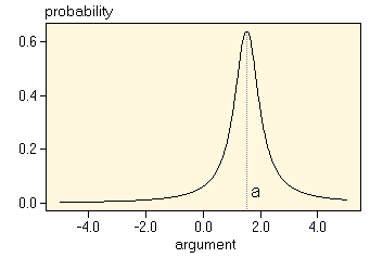 The graph at the left shows the probability density of a Cauchy distribution with the parameters a=1.5 and b=0.5 The graph at the left shows the probability density of a Cauchy distribution with the parameters a=1.5 and b=0.5 |
| Applications |
The Cauchy distribution occurs comparatively rarely. Examples of a Cauchy distribution:
- The ratio of two normally distributed random variables is Cauchy distributed.
- The Cauchy distribution arises in connection with the Brownian motion ("random walk") of molecules
|
| Mean |
The mean does not exist |
| Variance |
The variance does not exist |
| Simulation |

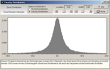 The program Cauchy Distribution calculates the probability density function of the Cauchy distribution and allows to calculate the mean as a function of the size of the sample. The following example has been calculated by using this simulation. The program Cauchy Distribution calculates the probability density function of the Cauchy distribution and allows to calculate the mean as a function of the size of the sample. The following example has been calculated by using this simulation.
|
Example
The following figure shows the average of means of Cauchy distributed random numbers as a function of n for n=1..500 (C(n), blue line). Since the probability density function of the Cauchy distribution has long tails, the odds for large values to occur are not negligible. This makes the mean jump considerably even when several hundred or thousand random numbers are averaged. The gray symbols show the individual random numbers, the red arrows indicate occasions where a random number exceeds the visible limits of the diagram.
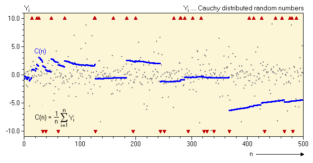
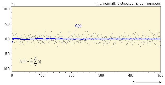
In contrast to the Cauchy distribution the mean of normally distributed data G(n) moves only slightly for n > 50 and the variation of the average decreases with increasing n. Thus the average can converge on the true mean of the distribution, since the probability of very small or very large numbers is so low that, on the long run, extreme values have no effect.
|

 Univariate Data
